How to make an attendance sheet using Excel

Personnel attendance monitoring is something that every company or unit is very concerned about. Let's explain how to use Excel to make a professional personnel attendance sheet.

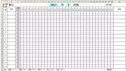
1. Open a blank EXCEL worksheet and draw it as shown below.

In the picture, M1:P1 are merged cells, used to fill in "year", S1:T1 are merged cells, used to fill in "month", set to light blue for eye-catching purpose Color shading.

2. In order to automatically display the "week" in the second row, you need to set a formula as follows:

Enter the formula =IF(WEEKDAY(DATE($M$1,$S$1,D3),2)=7,"Day",WEEKDAY(DATE( $M$1,$S$1,D3),2))

At this time, you can see a "day" representing the week appearing in cell D2 (this means that May 1, 2011 is Sunday).

Formula meaning: First use the DATE function to combine the "year" in the M1 cell, the "month" in the S1 cell, and the "day" in the D3 cell to form a "year" that can be recognized by the computer. "Date"; then use the WEEKDAY function to turn this "date" into the number represented by the week.

The parameter "2" is added after the WEEKDAY function to display Monday as "1", Tuesday as "2"... and Sunday as "7" .

Since we are not used to calling Sunday "Sunday 7", we finally use the IF function to make a judgment and automatically change the "7" displayed to "Day".

Tip: The functions DATE and WEEKDAY have detailed usage introductions in the help that comes with EXCEL. Friends who want to know about them can refer to them.

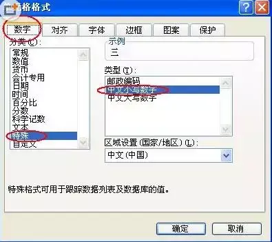
In order to facilitate the habits of us Chinese people, it is necessary to change the week shown as Arabic lowercase numerals into Chinese numerals, that is, "week 1" becomes "Monday" in this format. This needs to be achieved by defining the cell format.

Select cell D2, right-click "Format Cells", select the "Number" tab in the format window that appears, and select "Special" in the "Classification" box on the left , select "Chinese lowercase numbers" in the "Type" box on the right, and press "OK" to exit.

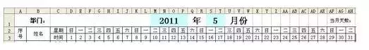
After completing this, you can use the mouse to select cell D2, hold down the "fill handle" in its lower right corner and drag to copy cell AH2. The effect is as follows:

In the AI ​​cell, you can use the formula to display the total number of days in the month, the formula =DAY(DATE(M1,S1+1,1)-1)

Formula meaning: First, use the DATE function "DATE(M1,S1+1,1)" to get the date on the first day of the next month of this month. In this example, this month is May, and the first day of the next month is June 1.

Then subtract 1 to get the date of the last day of the month, which is May 31, and finally use the DAY function to take out "31" indicating the number of days in the month.

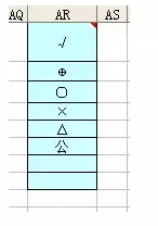
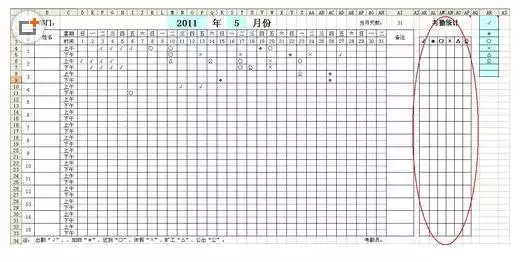
3. First set some attendance symbols and place them in the AR column, as shown in the figure:

These symbols are not uniformly stipulated. You can set them according to your habits and preferences, or they can be represented by Chinese characters. In short, just follow your own habits.

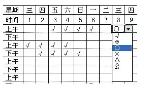
How to input these symbols into the D4:AH33 area of ​​the attendance sheet conveniently and quickly? We use the drop-down box method.

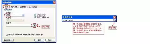
Select the D4:AH33 area, click "Data-Validity" in the toolbar above, the validity setting dialog box will pop up, select the "Settings" tab, and select "Allow" "Sequence", click the fold button on the right end of "Source", then use the mouse to select the AR1:AR8 area in the table, click the fold button again, return to the validity setting window, and press "OK" to exit.

After completion, when any cell in the D4:AH33 area of ​​the attendance sheet is selected, a drop-down box button will appear. Click the button to pop up the drop-down box, which can be conveniently selected with the mouse. Attendance symbol to be entered.

4. Attendance can be input. How to count everyone’s attendance? Or calculate statistics automatically through formulas.

First draw an area for attendance statistics, as shown in the red circle in the figure below:

Multiple merged cells need to be set in this area. AK4:AK5 is merged, AL4:AL5 is merged...AP4:AP5 is merged. That is to say, the upper and lower lines corresponding to each name need to be merged, so that it is convenient to count morning and afternoon in one grid.

After completing the merge operation of the AL4:AP5 area, select the fill handle in the lower right corner of the area, hold down the left mouse button and pull it down until you reach cell AP33 and then release the left mouse button. , you can quickly turn the following cells into a merged state. (In fact, it is a copy of the style of AL4:AP5)

Since the first person's attendance record area is the D4:AH5 area, it is necessary to count the number of attendance symbols in this area to know the attendance status of this person. .

First enter the attendance symbol in AK3:AP3, and then enter the formula =COUNTIF($D4:$AH5,AK$3) in cell AK4

Formula meaning: Use the COUNTIF function to count how many times the symbol in the AK3 grid appears in the D4:AH5 area.

Use the drag-and-copy function to copy this formula to the AK4:AP4 area.

Select the AK4:AP4 area, hold down the fill handle in the lower right corner of AP4 and drag it down to copy until it reaches cell AP33.

Now each cell in the statistical area has a formula. Since some parts of the formula use the absolute reference symbol "$", during dragging and copying, each cell The formulas in the cells are all different.

Tip: In this attendance sheet, the "drag and copy" method is used many times, which can greatly simplify the operations of entering formulas and setting formats, and can be used flexibly in formulas The absolute reference symbol "$" can also quickly input regularly changing formulas into the area, avoiding the trouble of inputting them one by one.

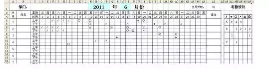
Now let’s take a look at the effect of statistical formulas

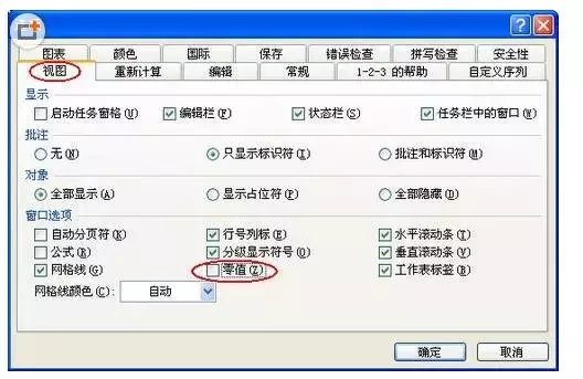
In the statistical results, there will be many 0 values ​​appearing, which means that the corresponding attendance symbols do not appear in the attendance area. When there are too many 0 values, it will feel "messy". We set to "hide" these 0 values.

Click "Tools-Options" in the toolbar, the options window will appear, set as shown below, and remove the check mark before "zero value" to prevent these 0 values ​​from being displayed. .

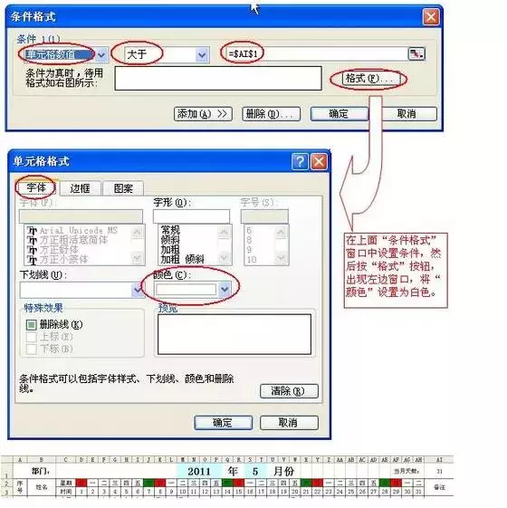
5. At this point, the attendance sheet is basically completed. Careful friends will find a small problem, that is, the three dates 29, 30, and 31 always appear in the three grids of AF3, AG3, and AH3, even when there are only 28 days in February, which is very unpleasant.

We can use conditional formatting to automatically display or hide them according to the change of the month. That is, the AH3 grid becomes blank when the month is small, and 31 is displayed when the month is large. If February is not a leap month, the numbers in the AF3, AG3, and AH3 cells will not be displayed.

Select the AF3:AH3 area, click "Format-Conditional Formatting", and set as shown below:

Using this conditional formatting method, you can also set the D2:AH2 area so that they turn into different colors on Saturday and Sunday, which can display the weekly situation more intuitively. Setting method You can think about it yourself.

The above steps for making an attendance sheet using Excel are basically of a general type and are suitable for use by many companies. You can also customize it according to your own situation.