Excel, By creating a "table", you can easily group and analyze data, and you can filter and sort the data in the "table" independently of the data in other rows and columns in the worksheet. In addition, "Table" also has some features that regular tables do not have, such as fixed title rows, automatic expansion of table areas, automatic filling of formulas, etc. Add-ins such as Power Query and Power Pivot also rely on "Table".
Next, the editor will lead you to learn about the "table" function of Excel 2019. In order to facilitate the distinction, except for the button names in the ribbon, other parts of the article are referred to as "super tables" to refer to this special "table".
Create a "super table"
The steps to create a "super table" are as follows.
❖ Select the object, which is the cell area to be generated as a "super table", as shown in Figure 1-1 The cell range A1:B9. If there are no empty rows or columns in the entire data area, you can select any non-empty cell (such as A4) as the selected object.
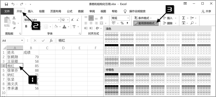
Figure 1-1 [Apply table format]
❖ Click the [Apply Table Format] drop-down button under the [Home] tab and select it in the extended menu Any table style, as shown in Figure 1-2.

Figure 1-2 [Insert] → [Table]
You can also click the [Table] button under the [Insert] tab, as shown in Figure 1-2. Or press the <Ctrl+T> or <Ctrl+L> key combination.
❖ Retain the default settings in the pop-up [Create Table] dialog box, and then click the [OK] button to generate "Super table", as shown in Figure 1-3.
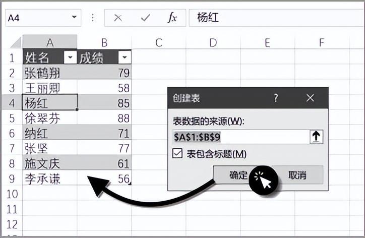
Figure 1-3 Generate "super table"
Features of "Super Table"
Super table has the following characteristics.
❖ There is one and only one header row. The content of the header row is in text format and has no duplication. The original field titles are duplicated. Yes, titles that appear multiple times will be distinguished by numbers.
❖ Automatically apply table styles.
❖ All merged cells are automatically unmerged, and the original content is in the first cell in the upper left corner of the original merged area. show.
❖ Select any cell in the "Super Table" and scroll down the worksheet, the table title automatically replaces the worksheet column label, as shown in Figure 1-4.
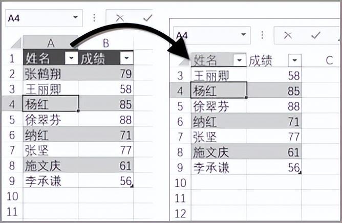
Figure 1-4 Scroll table, column headings automatically replace worksheet column headings
❖ The [Filter] button is automatically added to the title row, and a [Slicer] can also be inserted on the basis of the "Super Table" ] to quickly filter the data, as shown in Figure 1-5.

Figure 1-5 Insert [Slicer] on the "Super Table"
Changes in the application scope of "Super Table"
There is an application scope mark in the lower right corner of the "Super Table", as shown by the arrow in Figure 1-6. Use the mouse to drag and drop this mark. Markers can adjust the application scope of the "Super Table".
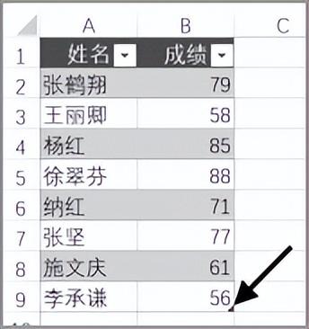
Figure 1-6 Application scope mark of "Super Table"
Another adjustment method is to click the [Adjust Table Size] button under the [Table Tools] [Design] tab, and in the pop-up [ Re-specify the table range in the Reset Table Size dialog box, as shown in Figure 1-7.
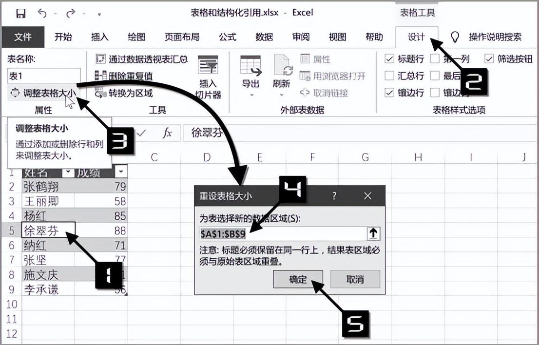
Figure 1-7 Adjusting the size of the "Super Table"
The application scope of "Super Table" can be automatically expanded to any area adjacent to "Super Table" on the right side or below of "Super Table" Enter content in a cell, and the size of the "Super Table" automatically expands to include the cells with the newly entered content. The newly expanded column will automatically add a title. If the original title content is [custom sequence], the new title content will be automatically generated according to the sequence rules. Otherwise, the default title of "column + number" will be automatically generated.
Clearing the contents of the entire row or column will not cause the scope of the "Super Table" to be automatically reduced. If you need to reduce the scope of the "Super Table", In addition to applying range markers and resizing the table by dragging and dropping with the mouse, you can also use the [Delete Column] or [Delete Row] functions.
Calculation of "super table"
1 Calculated column
"Super Table" enables the calculated column function by default.
If you enter a formula in any cell of the adjacent column on the right side of the "Super Table", the "Super Table" area will automatically expand and Apply the formula to all cells in the column, as shown in Figure 1-8.
For the newly added calculated column, a smart tag of [AutoCorrect Options] will appear. Users can modify the settings as needed, as shown in Figure 1-9 shown
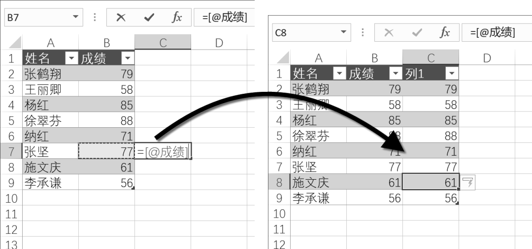
Figure 1-8 Formula automatically applied to a column
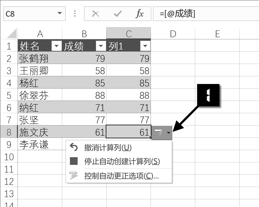
Figure 1-9 Autocorrect options
The table size of "Super Table" can automatically expand with the data. For example, if you create a PivotTable and a chart using SuperTable as the data source, when you add data to the SuperTable, the data source range of the chart and PivotTable will automatically expand accordingly.
If this function fails due to some misoperation, you can click [File] → [Options] to open the [Excel Options] dialog box. Then click [Proofing] → [AutoCorrect Options] to open the [AutoCorrect] dialog box. Under the [AutoFormat as You Type] tab, select the [Fill formula into table to create calculated columns] check box, and finally click the [OK] button, as shown in Figure 1-10.
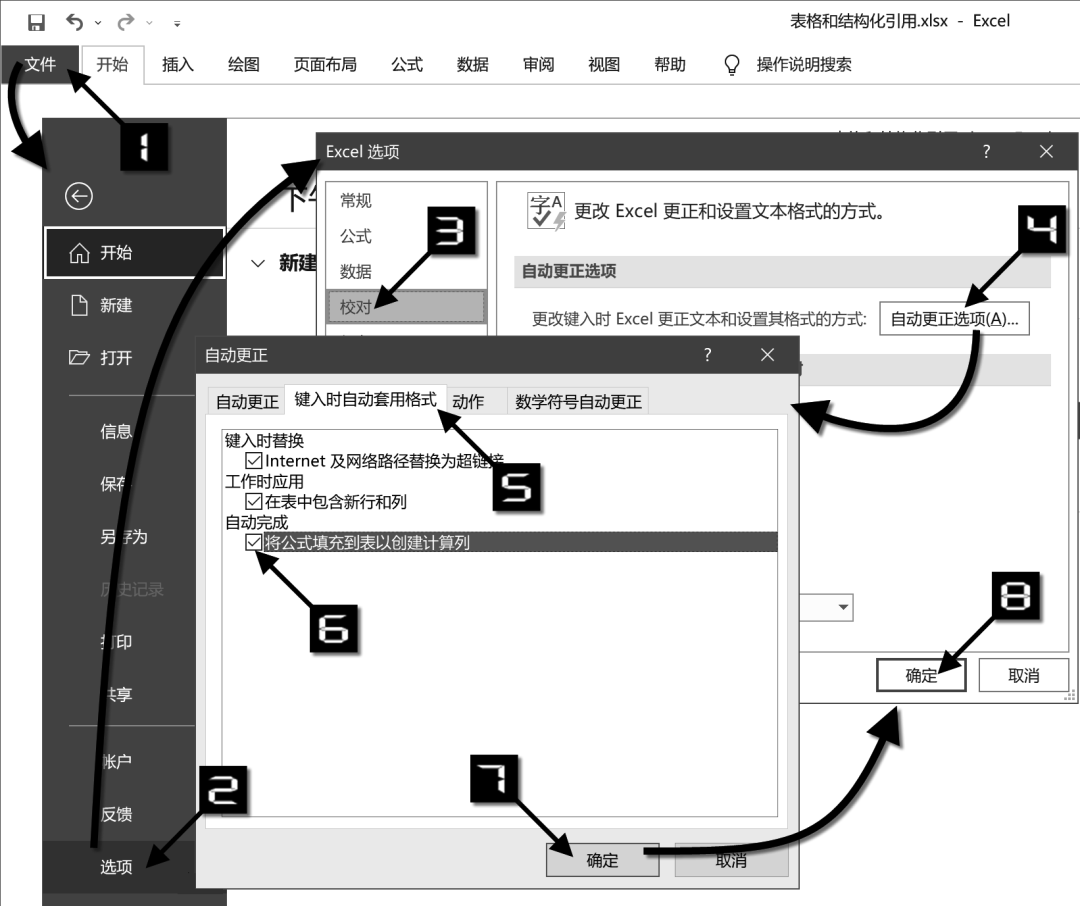
Figure 1-10 Turn on the calculated column function
2 Summary row
You can use the [Summary Row] function in "Super Table".
Select any cell in the "Super Table" and select the [Summary Row] checkbox under the [Design] tab of [Table Tools] , "Super Table" will automatically add a "summary" row, and the default summary method is summation, as shown in Figure 1-11.
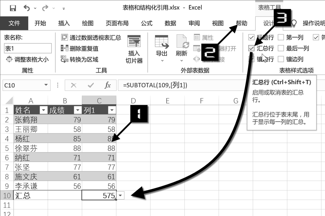
Figure 1-11 Summary row of "Super Table"
Click the cell in the summary row, a drop-down button will appear, you can choose different summary methods in the drop-down list, and Excel will automatically generate the corresponding The formula is shown in Figure 1-12.
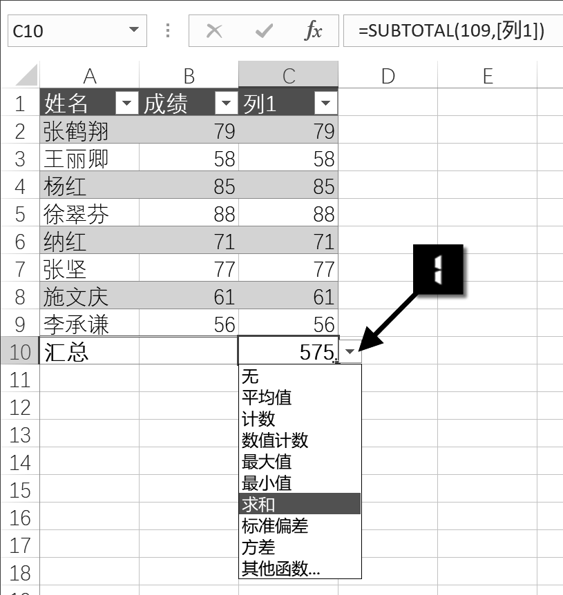
Figure 1-12 Select the summary method from the drop-down list
After adding a summary row, if you enter content in the lower cell adjacent to the "Super Table", the "Super Table" will not be automatically expanded. ” scope of application. At this time, you can click the cell of the last data record in the "Super Table" (the previous row of the summary row), such as cell C9 in Figure 1-12, and press the <Tab> key to add a new row to the table. Formula reference ranges in summary rows are also automatically expanded.
Through the above introduction, have you gained a deeper and systematic understanding of the "table" in Excel? It is easy to overlook the basics, but it is indispensable knowledge for learning Excel functions and formulas well.
Articles are uploaded by users and are for non-commercial browsing only. Posted by: Lomu, please indicate the source: https://www.daogebangong.com/en/articles/detail/ren-shi-Excel-biao-ge-de-te-dian.html
 支付宝扫一扫
评论列表(196条)
测试