030 Learn to make my own template
1) Click the "File" tab, click "New", there are 5 choices under "Available Templates", double-click "Blank Workbook" to create a new blank workbook Book, the shortcut key is Ctrl+N, contains 3 worksheets by default.
2) The other options are all borrowed. You can use "Sample Template", "My Template", "New Based on Existing Content", which are actually copies, such as this month's The attendance sheet can be copied from last month's, and this year's summary can be copied from last year's, and the content can be changed. Genuine users can also search for templates on the Office.com website.
3) Right-click on the label of the worksheet, you can also insert, "My Template" is under the "Common" tab, and "Sample Template" is under "Spreadsheet Solution". Now let's insert a "blood pressure monitoring" for reference.

Blood pressure monitoring template
4) We select columns A to G, click the arrow next to the border in the "Font" area of the "Home" tab to select all the borders, and you can see the text layout above. This design method using grid lines is very useful when designing web pages and slideshows, as it can ensure that the entire layout is neat and uniform. The first half is all about entering different text into different cell locations, just master it yourself.
5) Press Ctrl+Z to undo a step, right-click the cell where data needs to be entered, and select "Format Cells". In the "Border" category, these cells are set A gray underline and a middle dividing line are added between two juxtaposed boxes to make it easier to find the input position.
6) The date and time row below is the title row of the table. Because the "filter" function is used, the triangular arrow of the drop-down list box appears on the right side. For example, you can choose to display only the time by clicking on it. "Morning" or "Evening" data can also be sorted based on the selected column content. Click "Filter" in the "Sort and Filter" area of the "Data" tab to cancel and restore filtering.
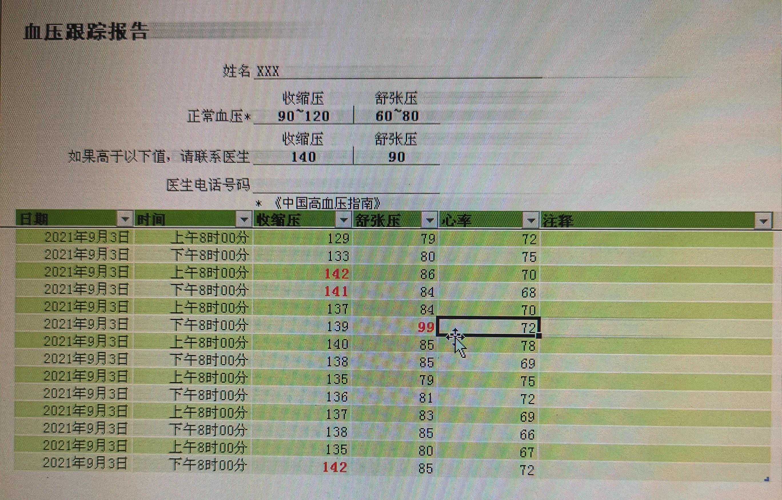
7) It is observed that there are three red numbers in the systolic blood pressure data, which means conditional formatting is applied. Click "Conditional Formatting" in the "Style" area of the "Home" tab, select "Manage Rules", and open the "Conditional Formatting Rule Manager". There are two rules. When "Cell Value > 140" in the D15:D28 area, the red font format is applied. We can select this one, click "Edit Rules" above, and "Edit Format Rules" will appear. You can see that the conditions are divided into three sections, here "=140", you can originally put the number in D10, use the cell reference to change it to "=$D$10", and enter 140 into D10 after confirmation.
8) The other diastolic blood pressure condition is processed similarly, "=90" is changed to "=$E$10", and 90 is entered into E10.
9) The automatic formatting of tables was discussed in the multiplication table. Click anywhere in the table and select your favorite style on the "Design" tab.
10) If you want to use China's hypertension standards, you can modify the text after the target blood pressure, warning blood pressure, and * accordingly.
11) Finally, select column C, change the number format to time format, enter the time value, and enter the number in the "00:00" format.
12) Then select "Excel Template" for "Save Type" in "Save As", give it a name, and the Chinese version of blood pressure monitoring was born.

The modified new version of the document
13) When creating new files in the future, this option will be available in "My Templates". According to your own preferences, you can adopt the principle of borrowing and transform other people's attendance sheets, timetables, course schedules, salary schedules, etc., and make them your own.
(to be continued)
Articles are uploaded by users and are for non-commercial browsing only. Posted by: Lomu, please indicate the source: https://www.daogebangong.com/en/articles/detail/mei-tian-xue-yi-dian-Excel2010-20-xue-zuo-yi-ge-wo-de-mu-ban.html

 支付宝扫一扫
评论列表(196条)
测试