- Picture and text skills
This function needs to be updated to the latest version of WPS Office
WPS Office official website: https://font2020.oss-cn-beijing.aliyuncs.com/wps/
Filter is a function that filters a series of data based on defined conditions. It consists of three parameters: an array, including null values.
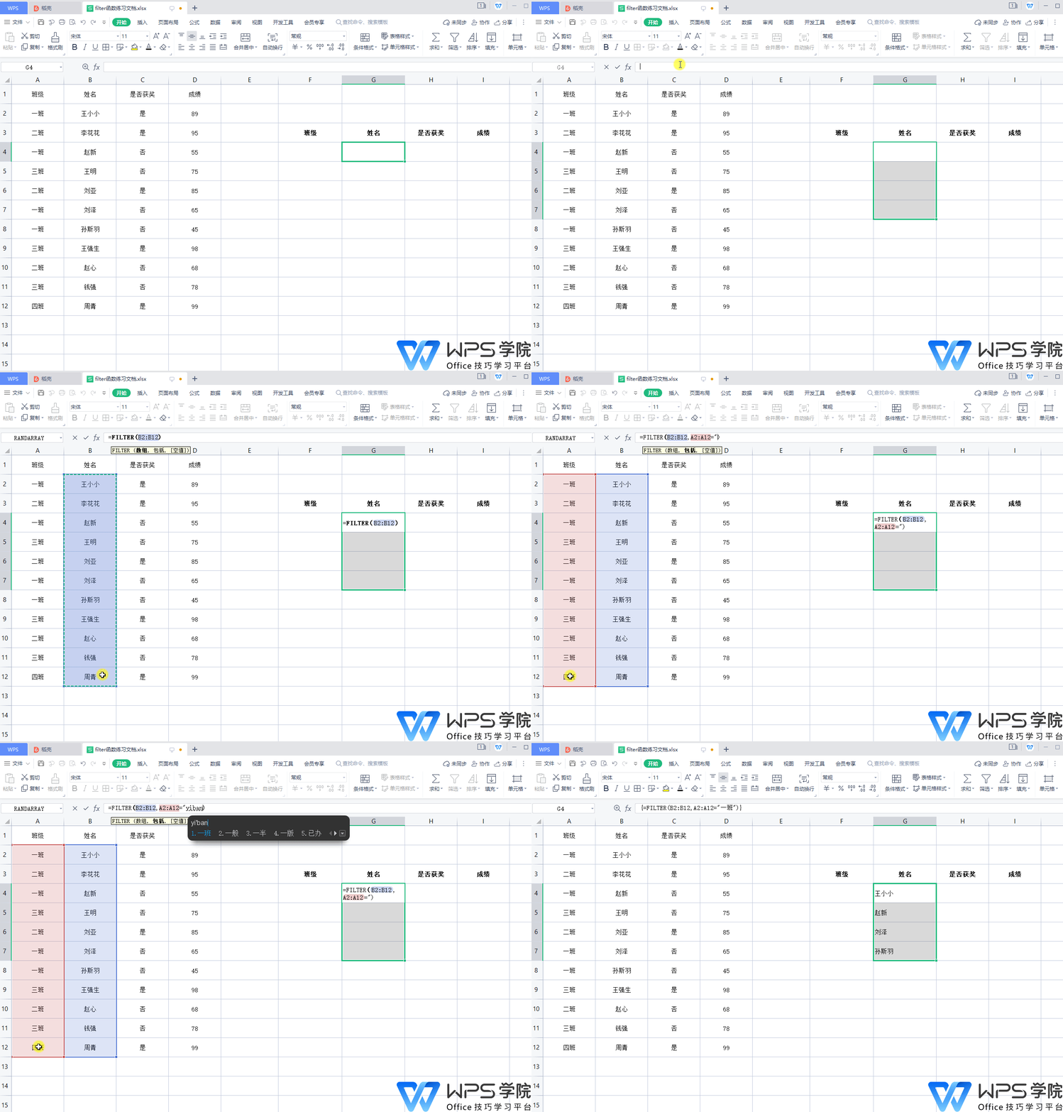
Take for example that we need to filter out the corresponding names by class in this table.

■First select the array return area, and then enter the formula =filter. Because we want to filter out names, enter the name column in the first parameter, and then the second parameter is The condition area means filtering names by class, so select the class column. After selecting the condition area, you must enter "="Class 1"" to filter out the corresponding names by class. You can leave the third parameter blank, then press "Ctrl+Shift+Enter" to confirm.
It should be noted that WPS Office does not currently support dynamic arrays, so you must use the "Ctrl+Shift+Enter" key shortcut to set it to array form. Other methods will only return a single value.

The FLITER function can also be combined with a multi-level drop-down list to create a table slicer effect.
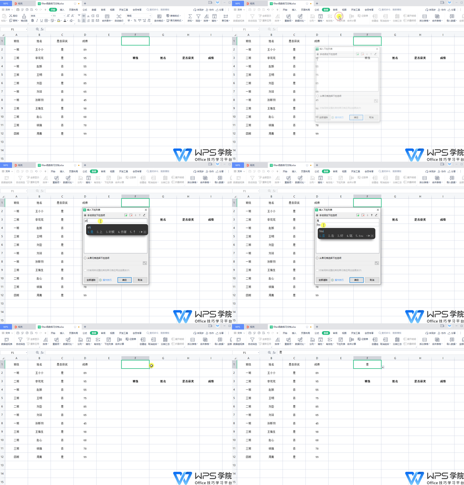
Take this table as an example. We hope to filter out all the information about the winners.
■Step 1: First create a second-level drop-down menu through the "Data" tab and "Drop-down List". Because the judgment conditions are relatively simple here, you can use manual addition. options. Other methods can be searched for "multi-level drop-down menu" in WPS Academy to learn.

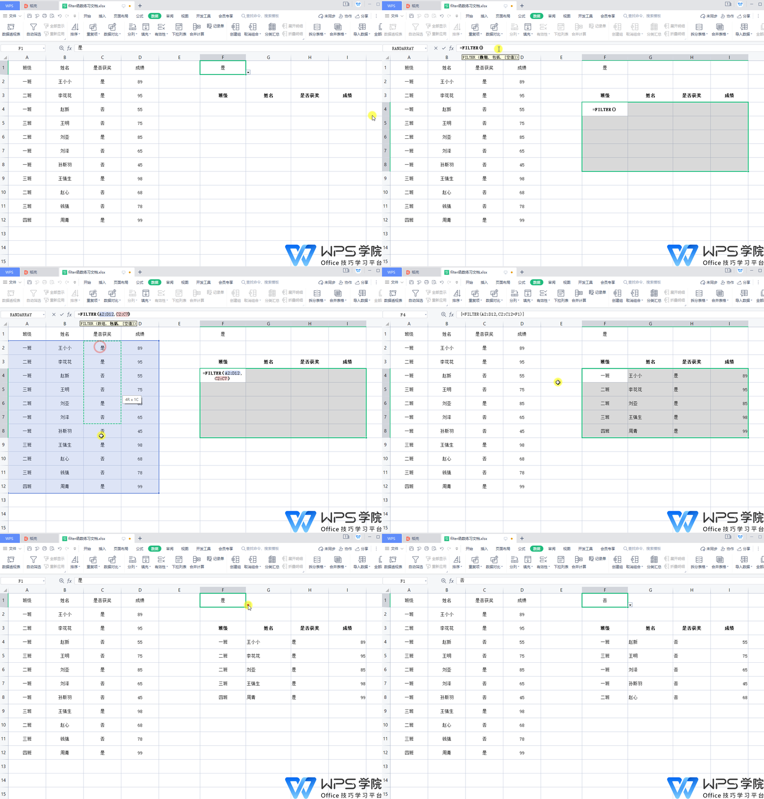
■Step 2: Select the return area, and then enter =filter. The first parameter selects the returned column, here is all, and the second parameter selects the condition column. Here, select whether to win the award column, enter =F1. It should be noted that the options in the drop-down list must be consistent with the options in the reference condition column. The third parameter can be ignored. Press "Ctrl+Shift+Enter" to confirm. At this time, click on the right side of cell G1 The drop-down list button allows you to filter student-related information based on whether you have won an award.

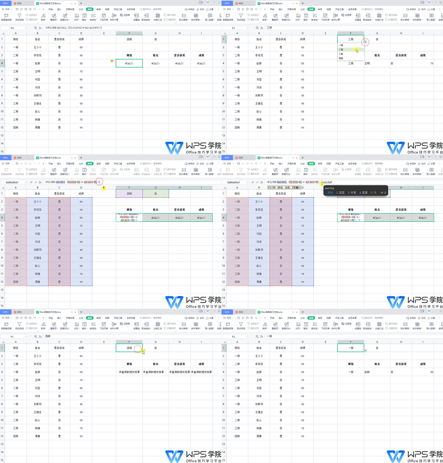
■FinallyWhen using theFILTER function to filter multiple conditions, a #CALC error value will appear. This is an error value returned because the result of the query based on the conditions is a null value. To handle this error, you need to use the third parameter of FILTER.
For example, we Add the third parameter to the entered formula. The third parameter is a customizable description of the null value result. For example, here we enter "No relevant results were found" and then confirm. At this point the error value becomes a defined text description. Note: All symbols in the formula need to be entered using the English input method.

Articles are uploaded by users and are for non-commercial browsing only. Posted by: Lomu, please indicate the source: https://www.daogebangong.com/en/articles/detail/cha-zhao-he-yin-yong-han-shu-ru-he-shi-yong-FILTER-han-shu.html

 支付宝扫一扫
评论列表(196条)
测试