- Picture and text skills
This function needs to be updated to the latest version of WPS Office
WPS Office official website: https://font2020.oss-cn-beijing.aliyuncs.com/wps/
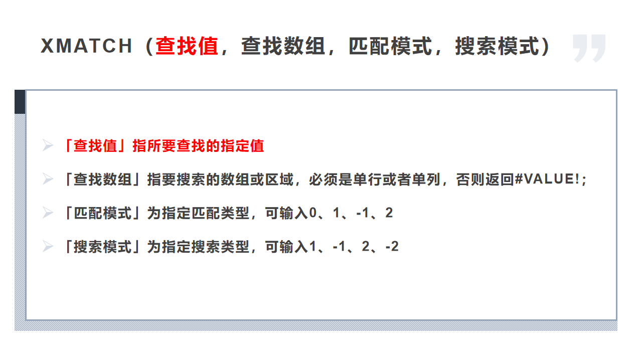
The XMATCH function can search for a specified item in an array or cell range, and then return the relative position of the item.
Its function syntax is XMATCH (find value, find array, match pattern, search pattern)

1. XMATCH function returns positions in batches
Take this table as an example. We want to return the product serial numbers of Table 2 in batches.
Select the cell range E3:E7 and enter the formula =XMATCH() in the formula edit bar
Enter the value or range you want to find in "Find Value", enter D3:D7;
Enter the array or area to be searched in "Search Array", enter B3:B11;
Enter the matching type in "Matching Pattern", enter 0 for a complete match;
Finally, use the shortcut keys Ctrl+Shift+Enter to fill this formula into the table in the form of an array.
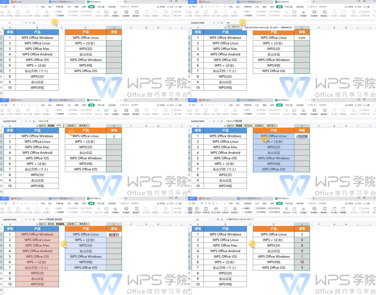
The meaning of this formula is to use the XMATCH function to find the product serial number corresponding to Table 1, and fill it into Table 2 in batches.
2. Matching mode of XMATCH function
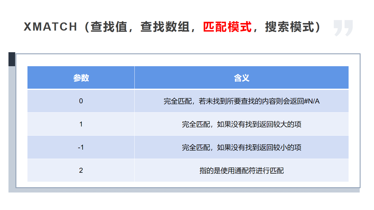
The parameters of "matching pattern" are as shown in the table:
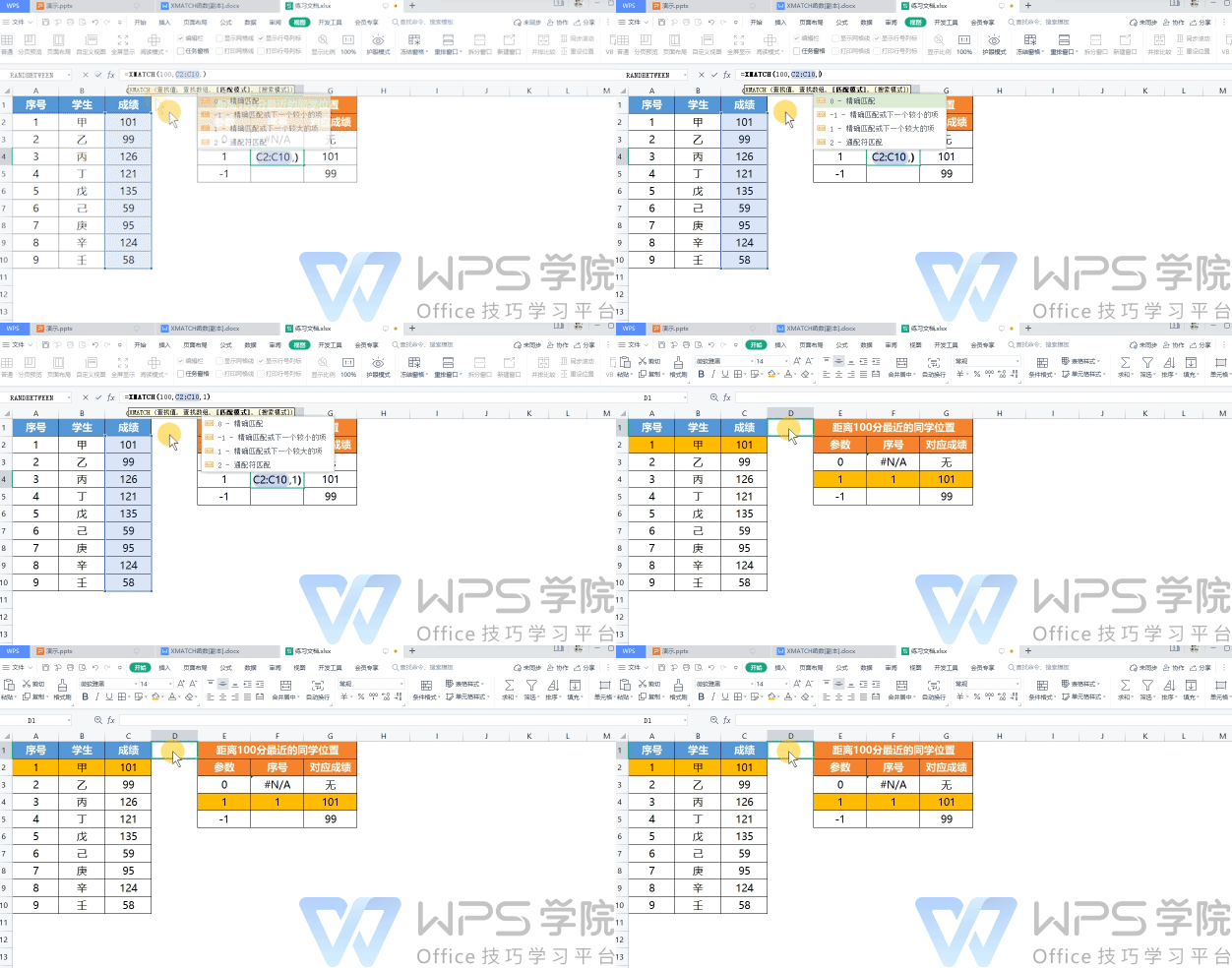
Take this table as an example, if we want to find the location of the closest student with 100 points.
Click the "Formula"-"Insert Function" button and find the XMATCH function,In "Find value" and enter it100;
Enter C2:C10 in "Search Array", that is, the value in the C2:C10 area is 100 points;
In "Match Mode", you can enter 0, 1, -1, 2:
Enter 0 for an exact match. When 100 points are not found in the transcript, #N/A will be returned;
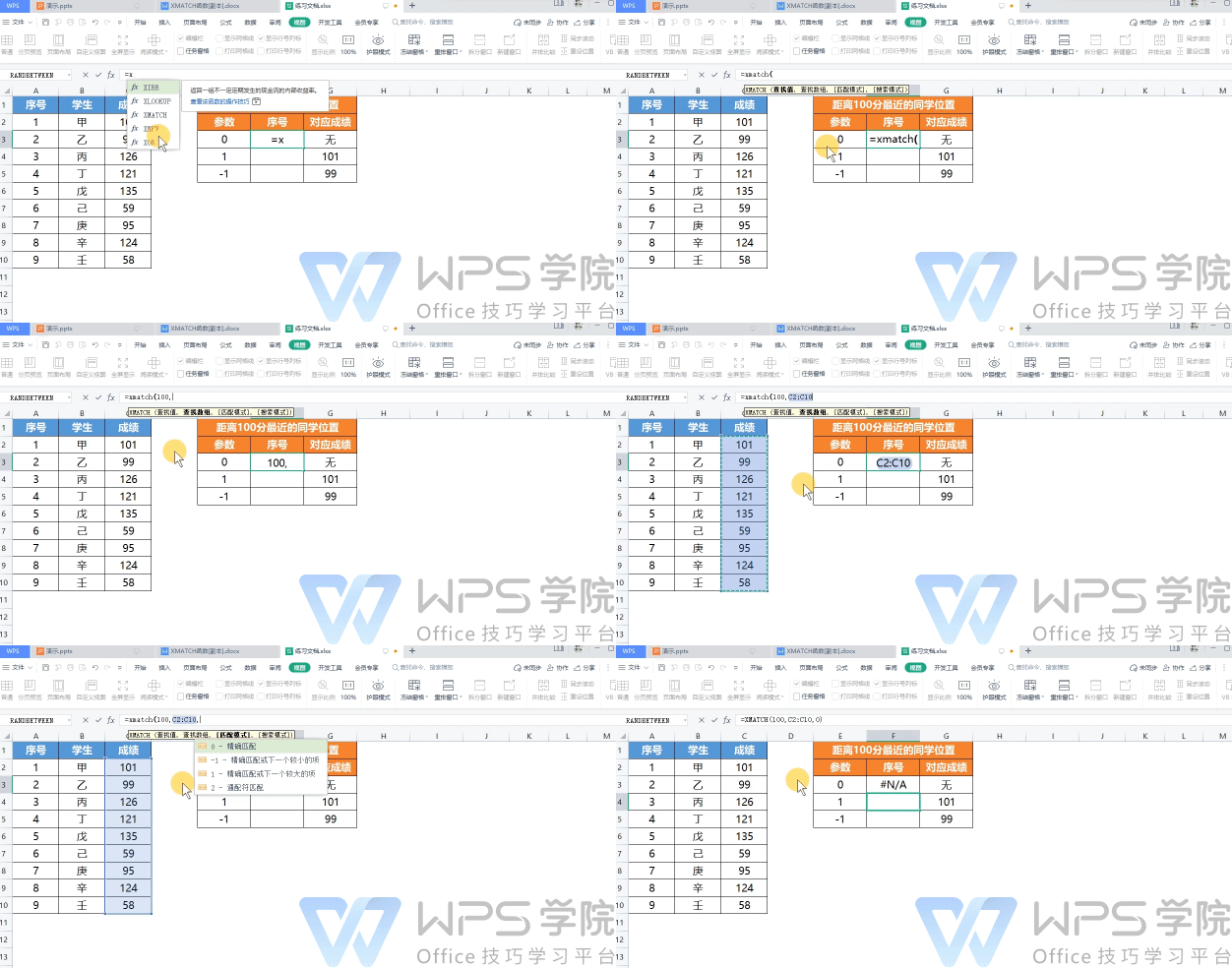
Enter 1 to match the next largest item.
When 100 points are not found in the transcript, the closest and largest score number to 100 points is returned, which is the number of 101 points;
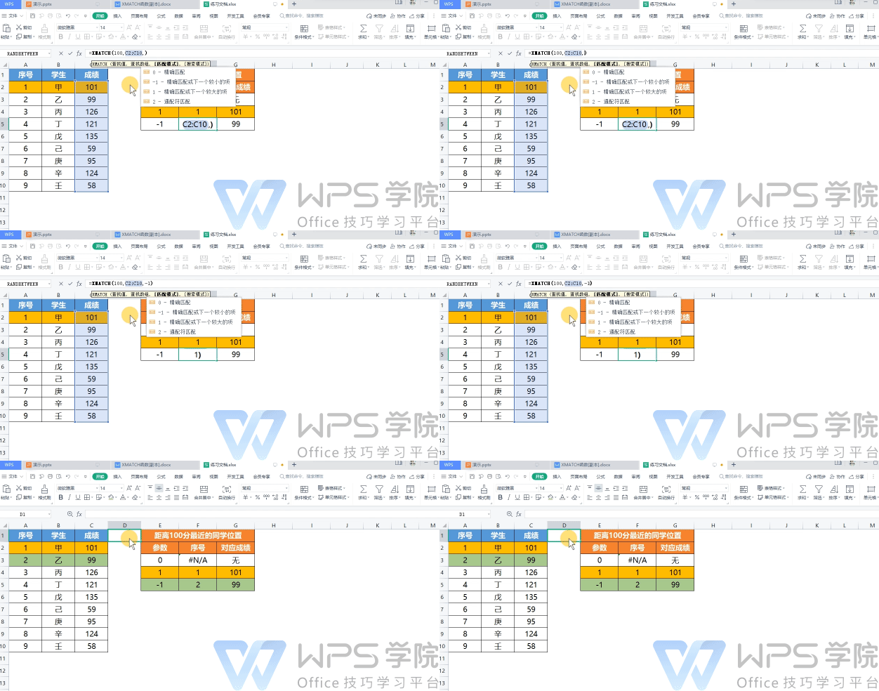
Enter -1 to match the next smallest item.
When 100 points are not found in the transcript, the closest and smallest score number to 100 points is returned, which is the number of 99 points.
3. Search mode of XMATCH function
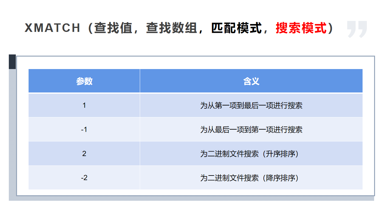
"Search mode" parameters are shown in the table:
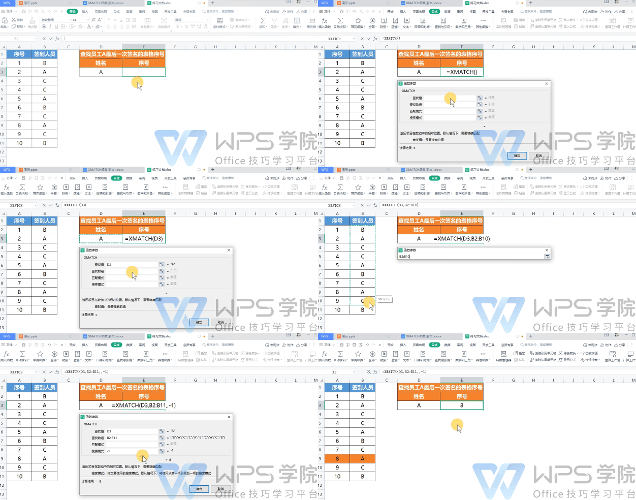
Take this employee sign-in form as an example. If you want to find the form serial number of employee A's last signature.
Enter D3 in "Find Value", which is the cell where employee A is located;"Search Enter "Array"B2:B11;
"Search mode" output -1, that is, search in reverse order;Click OK to return The form serial number of employeeA's last signature.
4. Combination of XMATCH function and INDEX function
The XMATCH function is often combined with the INDEX function. The INDEX function can return the contents of the specified row number and column number.
For a detailed explanation of the INDEX function, you can search for the keyword "INDEX" in "WPS Academy" to learn more.
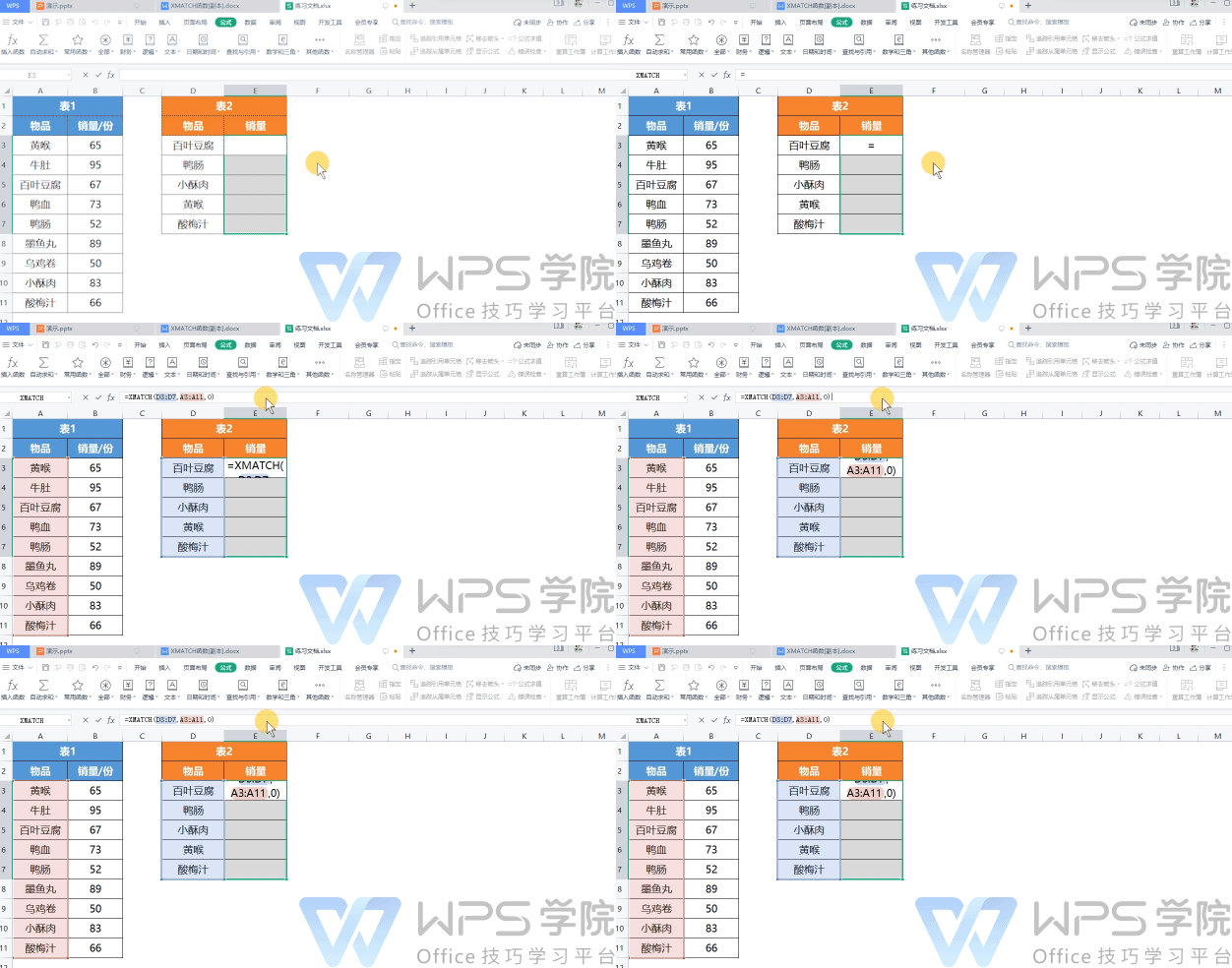
Take this table as an example. If we want to find the sales volume of items in Table 2, enter =XMATCH(D3:D7,A3:A11,0)
That is, use the XMATCH function to obtain the row number position of the item area of Table 2 in the item area of Table 1 in batches.
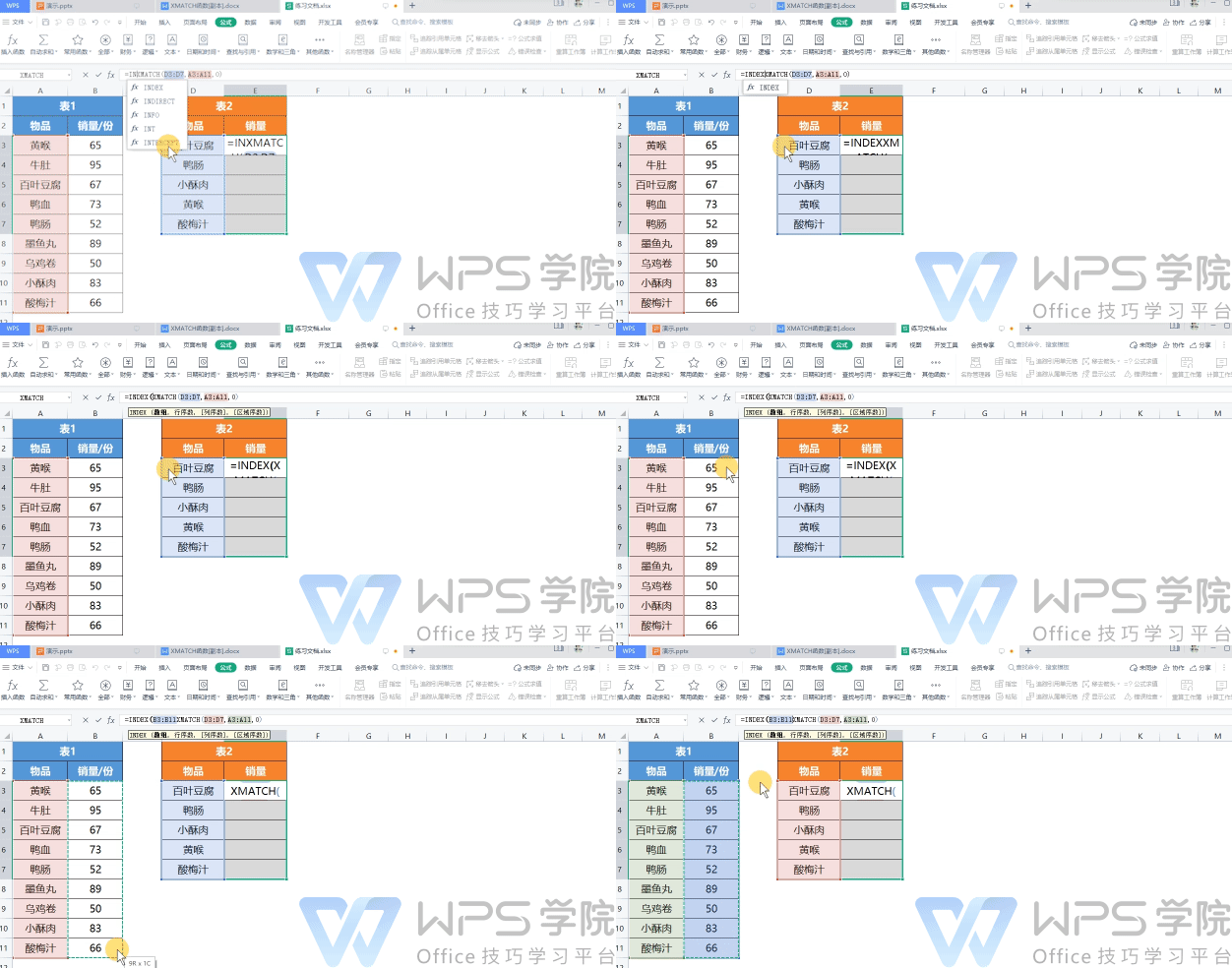
Then add the formula before the XMATCH function as =INDEX(B3:B11,XMATCH(D3:D7,A3:A11,0)), which means using the INDEX function, according to XMATCH The row serial number data obtained by the function is used to obtain the column data corresponding to Table 1.
Finally use the shortcut keyCtrl+Shift+Enter to fill this formula into the table in the form of an array middle.
Articles are uploaded by users and are for non-commercial browsing only. Posted by: Lomu, please indicate the source: https://www.daogebangong.com/en/articles/detail/cha-zhao-he-yin-yong-han-shu-XMATCH-han-shu-de-shi-yong-fang-fa.html

 支付宝扫一扫
评论列表(196条)
测试