When it comes to resolution, we naturally think of the resolution of the image. The higher the resolution, the clearer the displayed image and the more realistic the details.

Figure 1 Different resolution images

In spectrum analysis, there is also the concept of "Resolution-Resolution"!

Resolution is a basic concept in signal processing, including frequency resolution and time resolution.

Figuratively speaking, the frequency resolution is the width of the frequency seen when observing the spectrum through a frequency domain window function; the time resolution is the time width seen when observing the signal through a time domain window function. Obviously, the narrower such a window function, the better the corresponding resolution.

Figure 2 Garfield through the window "function"

In fact, such a statement is not vivid!

So let's not talk about the concept of resolution here, but first look at a classic example.

Look at an example first

There exists a time signal x(t) whose highest frequency is fc and does not exceed 3Hz.

Now sample it with a sampling rate of fs=10Hz, ie Ts=0.1s. According to the sampling theorem, the aliasing problem should not occur.

Let the duration of the signal x(t) be T, T=25.6s. Then the number of sampling points is T/Ts=256, that is, the number of points of x(n) obtained by sampling is 256.

Well, the above are some basic conditions.

Now the signal x(t) consists of three sinusoids whose frequencies are f1=2Hz, f2=2.02Hz, f3=2.07Hz, namely

xt=sin(2*π*f1*t)+sin(2*π*f2*t)+sin(2*π*f3*t);

Draw the waveform of xt as follows:

Figure 3 Waveform of signal x(t), duration 25.6s

x(t) consists of three frequencies f1\f2\f3, so when you observe its spectrum, you should be able to see three frequency components.

Now we calculate the DFT for x(t) and get the spectrum of x(t) as follows:

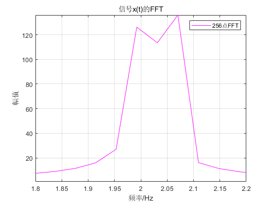
Figure 4 Spectrum of signal x(t), N=256

Since x(n) has 256 points, do a DFT operation with N=256 points.

According to Figure 4, we found that there are frequency components at f3=2.07Hz, but the f1 and f2 frequency components cannot be distinguished!

| looks like f1 and f2 are "fused" together |

At the same time, there are "significant" peaks at f1=2Hz, f2=2.02Hz, are the two frequency components lost?

Now we increase the duration T of x(t) to equal 102.4s.

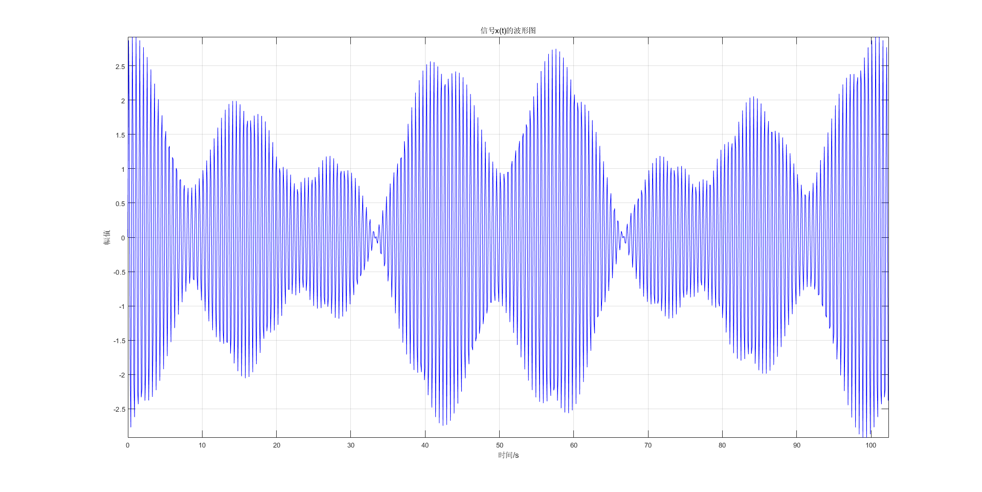
Figure 5 Waveform of signal x(t), duration 102.4s

Keep the sampling rate fs unchanged, then there are a total of N=1024 points, and other parameters remain unchanged. At this time, calculate the spectrum of the signal x(t) again

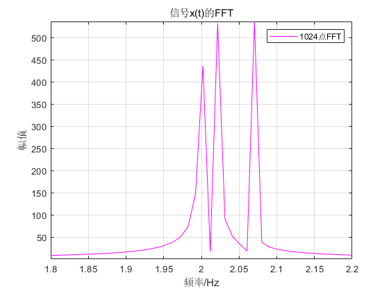
Figure 6 Spectrum of signal x(t), N-1024

Now the waveform is in line with my expectation, there are obvious "peaks" at f1=2Hz, f2=2.02Hz, f3=2.07Hz.

Why do we increase the duration T of the signal x(t), expand the number of FFT points N, and make the spectrogram more refined, so that we can "distinguish" 3 components?

Today's topic - resolution

Resolution is a basic concept in signal processing course, it includes frequency resolution and time resolution, here we focus on the former.

Frequency resolution can be defined in two ways:

1. The ability of an algorithm (such as spectrum analysis method, power spectrum estimation method, etc.) to keep two spectral peaks close to each other in the original signal, that is, the physical resolution ;
2. When performing DFT, the minimum frequency interval that can be obtained on the frequency axis is commonly referred to as the calculation resolution. Generally speaking, the frequency resolution refers to the physical resolution.

First of all, it is necessary to clarify the relationship between DTFT and DFT. DTFT is the Fourier transform of a discrete time sequence, which maps the sequence to a continuous normalized frequency domain;

DFT is the discrete Fourier transform of discrete time series, which maps the sequence into a discrete frequency sequence.

DTFT is a transformation with physical meaning, DFT is a tool for approximate calculation of DTFT, and FFT is just a fast algorithm of DFT.

In the end, the DFT result we see is composed of two parts, one part is the DTFT result of the signal with physical meaning, and the other part is the error signal caused by the analysis method (windowing, zero padding, etc.).

Physical resolution refers to the ability to distinguish between two spectral peaks that are close together, which can be represented by F0. Generally speaking, when the time-domain sampling rate fs is constant, the longer the signal length T, that is, the more sampling points N, the The higher the physical resolution is. with this relationship:

where Ts is the time domain sampling interval.

It should be noted that this refers to the real actual signal length, and the number of sampling points also refers to the number of sampling points on this length, not the length or number of sampling points after zero padding.

| That is to say, the physical resolution F0 only depends on the length of the time domain signal |

Calculation resolution refers to the distance between every two spectral lines obtained by doing point DFT for a point sequence, which is F0'.

And here is no longer the actual number of points, but the point when calculating DFT. If it is zero-filled, it will be the number of points after zero-filling.

In the MATLAB program, the physical resolution is the actual resolution, but what we see is the result after DFT, that is, the calculation resolution.

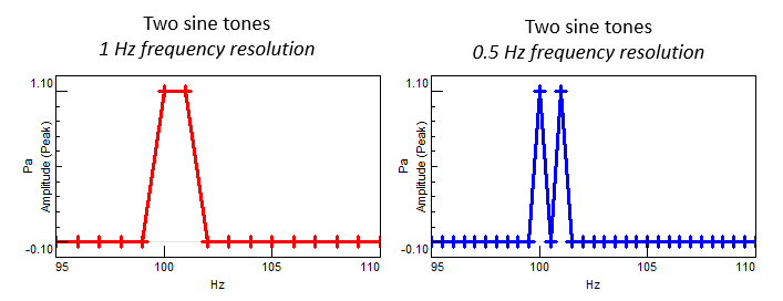
Figure 7 Spectrum of different resolutions

So, when the physical resolution is high enough, we can properly increase the calculation resolution, so that the invisible spectral components can be seen. However, when the length of the time-domain signal is insufficient, the physical resolution is low, and no matter how much the calculation resolution is improved, it will not help.

Go back to the example at the beginning of the period

When the length T of the signal x(t) is determined to be 25.6s, and the sampling frequency fs=10Hz, the physical resolution is fixed at this time, as

F0=1/T=fs/N=0.0391Hz

The signal x(t) has three frequency components, and f2-f1=0.02<F0, so the sine component produced by f2 cannot be distinguished at this time; and because f3-f1>F0, the sine component produced by f3 can be distinguished portion.

According to the above conclusions, the physical resolution only depends on the length of the time domain signal, so the expansion time T is 102.4s, and the sampling frequency remains unchanged, that is, the number of points N=1024 is increased.

Physical resolution at this time

F0=1/T=fs/N=0.0098Hz

At this point, three frequency components f1, f2, and f3 can be distinguished.

Now the physical resolution meets the requirements and is equal to the calculated resolution.

Steps and methods of DFT/FFT parameter selection:

If the highest frequency fc of the signal is known, in order to prevent aliasing, the selected sampling frequency fs satisfies

fs≥2fc

Then according to actual needs, select the frequency resolution F0, once F0 is selected, you can determine the number of points N required for DFT, that is

N=fs/F0

We hope that the smaller F0 is, the better, but the smaller F0 is, the larger N is, and the amount of calculation and storage will increase accordingly.

And we want N to be an integer power of 2. If the data of N points has been given and cannot be increased, we can make N an integer power of 2 by padding with zeros.

After fs and N are determined, the length of the required corresponding analog signal x(t) can be determined, that is,

T=N/fs=NTs

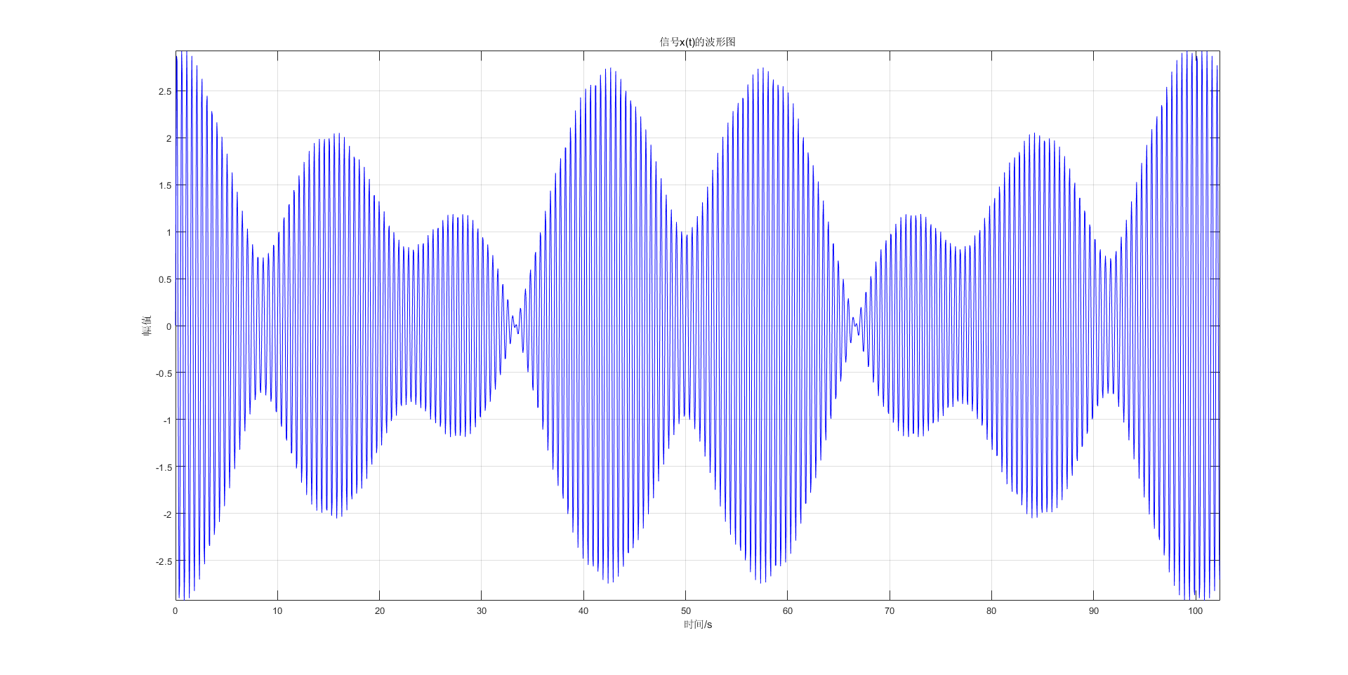
Figure 8 Waveform of signal x(t), duration 102.4s, sampling points 2048

It has been pointed out before that the resolution F0 is inversely proportional to T, not N, so in the case of a given T, increasing N by reducing Ts cannot improve the resolution.

This is because T=NTs is a constant, if Ts is reduced by m times, N is also increased by m times, then

F0=mfs/mN=fs/N=1/NTs=1/T

That is, F0 remains unchanged.

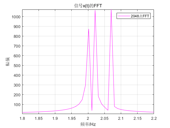
Figure 9 Waveform of signal x(t), N=2048

In Figure 8, we increase the sampling frequency fs so that there are 2048 sampling points.

According to the above conclusions, the spectral resolution will not change. It can be clearly seen from Fig. 9 that the frequency spectrum has not changed compared to Fig. 6 .

Conclusion

To sum up, we have noticed that in Matlab, when using the fft function for spectrum analysis, you must figure out the spectrum resolution you need, and then choose the appropriate time duration and sampling rate. Otherwise, if the spectrum analysis is carried out muddle-headedly, a lot of information may be missed in the spectrum image obtained.

Welcome to like, leave a message in the comment area to communicate.

For more exciting communication/signal processing content, welcome to join the "Squad Leader Communication School"